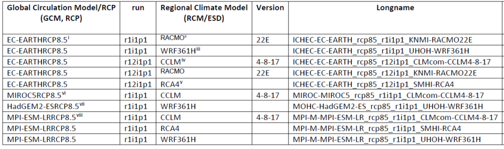
Below, we provide insights of the data and methodologies used for the Baden-Württemberg climate portal. The raw data were provided by the State Institute for the Environment Baden-Württemberg (LUBW).  It consists of a ten-member ensemble, from  a combination of six global models (GCM) and four regional models (RCM) (Fig. 1). The modelling was carried out within the EURO-CORDEX (https://euro-cordex.net/) (Jacob et al., 2014) and ReKliEs-De (https://reklies.hlnug.de, Huebner et al., 2017) projects. The BIAS adjustment and interpolation to a 5×5 km grid (of ~12.5 km) was performed by the German Weather Service (DWD) (https://www.dwd.de) (Brienen et al., 2020). The models were subjected to a plausibility check following the example of the Bavarian State Office for the Environment (LfU, 2020), and evaluated by LUBW for the state of Baden-Württemberg. The models are based on the RCP8.5 scenario (Moss et al., 2010), which assumes strong climate change in the absence of effective climate protection measures. Further information on the data basis can be found in the Klimaleitplanken 2.0 (LUBW, 2021a).

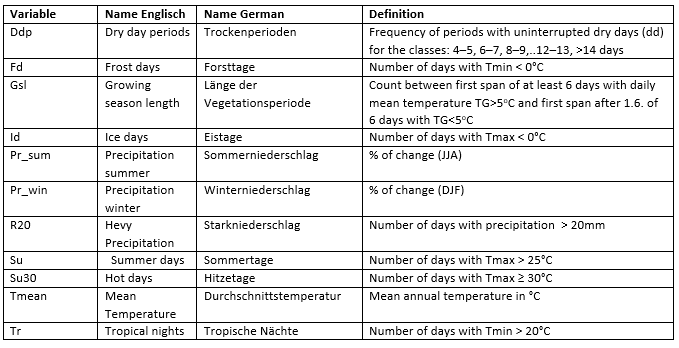
A total of 11 climate indices were derived from the above regional climate models (Fig. 2), which were calculated as 30-year averages for three different time periods. These are the climate normal periods 1971-2000 (reanalysis), 2021-2050 (near future) and 2071-2100 (far future). In particular, the minimum, maximum and 50th percentile of the model ensemble was analysed in greater detail for these periods.

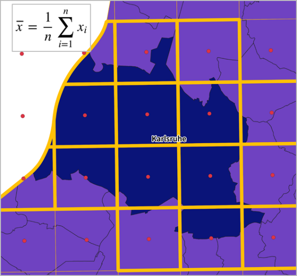
The data were available as tables with regularly arranged coordinates in a 5 km grid. The centroids of this point grid were transferred into a regularly arranged grid so the data could be spatially represented and analysed. In order to be able to make a statement for the municipal level, all overlapping grid cells per municipality area were aggregated by averaging (Fig. 3).  This can lead to zoning effects. From a modelling perspective, there are therefore limits to spatial aggregation (LUBW 2021b).  Nevertheless, in terms of user-friendliness, the advantages resulting from the transfer to known reference areas (here: municipal area) outweigh the disadvantages (here: minor deviations from the point grid). The model-related uncertainties are taken into account by showing the mean value of the model ensemble (50th percentile) as well as the variability range (minimum and maximum).

In addition to the range of variation, arrows are used to indicate the change in values compared to the actual situation 1971-2000, as well as the ranking in a state-wide comparison (Fig. 4). The change in direction is indicated if at least 7 out of 10 models of the ensemble agree. This corresponds to the assessment level “likely” according to the IPCC standard (Mastrandrea et al., 2011). If less than 7 out of 10 models show the same directional change, this is indicated as “unclear”.

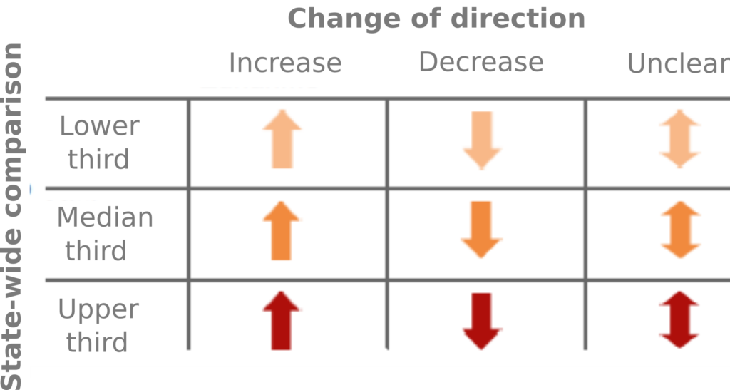
The colour levels of the arrows indicate the change in each indicator in three categories. The colour level indicates how the respective indicator compares to all other municipalities in Baden-Württemberg. The highest absolute values are assigned to the “upper third”, the lowest values to the “lower third”. The classification of the class boundaries was carried out separately for each indicator and each time period according to the algorithm of Jenks & Caspall (1971).

For further inquiries, please contact Nils Riach.

Literature

Brienen, S.; Walter, A.; Brendel, C.; Fleischer, C.; Ganske, A.; Haller, M. et al. (2020): Klimawandelbedingte Änderungen in Atmosphäre und Hydrosphäre: Schlussbericht des Schwerpunktthemas Szenarienbildung (SP-101) im Themenfeld 1 des BMVI-Expertennetzwerks, zuletzt geprüft am 08.07.2021.

Huebener, Heike; Hoffmann, Peter; Keuler, Klaus; Pfeifer, Susanne; Ramthun, Hans; Spekat, Arne et al. (2017): Deriving user-informed climate information from climate model ensemble results. In: Adv. Sci. Res. 14, pp. 261-269. doi: 10.5194/asr-14-261-2017.

Jacob, Daniela; Petersen, Juliane; Eggert, Bastian; Alias, Antoinette; Christensen, Ole Bøssing; Bouwer, Laurens M. et al. (2014): EURO-CORDEX: new high-resolution climate change projections for European impact research. In: Reg Environ Change 14 (2), pp. 563-578. DOI: 10.1007/s10113-013-0499-2.

Jenks, G. F., Caspall, F. C., 1971. “Error on choroplethic maps: definition, measurement, reduction”. Annals, Association of American Geographers, 61 (2), 217-244.

LfU (ed.) (2020): Das Bayerische Klimaprojektionsensemble – Audit und Ensemblebildung. Bavarian State Office for the Environment.

LUBW (2021a): Klimazukunft Baden-Württemberg – Was uns ohne effektiven Klimaschutz erwartet! Ed. by Landesanstalt für Umwelt Baden-Württemberg.

LUBW (2021b): Nutzungshinweise für die Verwendung von Klimamodellauswertungen für Baden-Württemberg. Ed. by Landesanstalt für Umwelt Baden-Württemberg.

Mastrandrea, Michael D.; Mach, Katharine J.; Plattner, Gian-Kasper; Edenhofer, Ottmar; Stocker, Thomas F.; Field, Christopher B. et al. (2011): The IPCC AR5 guidance note on consistent treatment of uncertainties: a common approach across the working groups. In: Climatic Change 108 (4), pp. 675-691. DOI: 10.1007/s10584-011-0178-6.

Moss, Richard H.; Edmonds, Jae A.; Hibbard, Kathy A.; Manning, Martin R.; Rose, Steven K.; van Vuuren, Detlef P. et al. (2010): The next generation of scenarios for climate change research and assessment. In: Nature (463), pp. 747-756. DOI: 10.1038/nature08823.